|
| Place of Origin: | America |
| Brand Name: | TYCO |
| Certification: | CE |
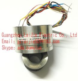
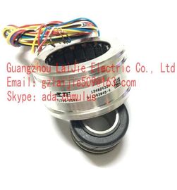
| Model Number: | V23401-H2010-B202 |
| Minimum Order Quantity: | 1pcs |
|---|---|
| Packaging Details: | carton |
| Delivery Time: | in stock |
| Payment Terms: | T/T, Western Union, MoneyGram |
| Supply Ability: | 10000pcs/week |
| TYCO: | TYCO | V23401-H2010-B202: | V23401-H2010-B202 |
|---|---|---|---|
| America: | America | Color: | Black |
| Temperature: | 20-120 | Wire: | Wire |
| Material: | Iron |
Guang Zhou Lai Jie Electric Co.,LTD
Please contact with “Tommy” for the price
V23401-H2010-B202
V23401-H1005-B101
V23401-T1005-B102
V23401-H1005-B102
V23401-T1009-B114
V23401-H1009-B114
V23401-T1009-B122
V23401-H1009-B122
V23401-T1009-B101
V23401-H1009-B101
V23401-T1009-B102
V23401-H1009-B102
V23401-T2001-B214
V23401-H2001-B214
V23401-T2001-B222
V23401-H2001-B222
V23401-T2001-B201
V23401-H2001-B201
V23401-T2001-B202
V23401-H2001-B202
V23401-T2009-B214
V23401-H2009-B214
V23401-T2009-B222
V23401-H2009-B222
V23401-T2009-B201
V23401-H2009-B201
V23401-T2009-B202
V23401-H2009-B202
![]()
![]()
![]()
The acquisition and archiving cycles in Tag Logging are based on previously configured times. Frequently used time cycles are already created by WinCC when you create a new project. You can configure additional time cycles as needed. WinCC distinguishes between cycle times and time series
A new cycle time is calculated on a basis that is multiplied with an integer factor. Cycle times are independent of the current time. The acquisition and archiving based on a cycle time is started as configured and repeated cyclically thereafter. Basic cycles are: ● 1 day ● 1 hour ● 1 minute ● 1 second ● 500 ms (half a second)
Time series are based on the calendar. The acquisition and archiving based on a time series takes place daily, weekly, monthly or annually. The day can be specified as day of the week or fixed calendar date. The time of the acquisition or archiving on the respective day can either be specified or depend on the system start.
. Click on . The updated display is stopped. 2. While holding the left mouse button down, move the cursor in the desired direction in the trend window. The displayed area in the trend window is adapted on the time axis and on the value axis. 3. Clicking on again will restore the original trend window view.. Click on . The updated display is stopped. 2. While holding the left mouse button down, move the cursor in the desired direction in the trend window. The displayed area in the trend window is adapted on the time axis and on the value axis. 3. Clicking on again will restore the original trend window view.
The cyclical acquisition and archiving cycles are based on these timers. Frequently used time intervals are provided by WinCC when you create a new project. If you wish to use timers that deviate from these standard timers, you can configure new timers. A new time cycle is calculated on a basis that is multiplied by an integer factor: Cycle time = time factor x time basis
Select the "Cycle times" folder under the "Timers" folder in the navigation area of the "Tag Logging" editor. All configured time cycles are displayed in the table area. You can use these time cycles to configure the acquisition and archiving cycles. 2. To create a new timer, click the top empty cell and enter a name in the "Timer name" column of the table area. A new timer is created. 3. Edit the properties of the timer in the "Properties" area.
Time series are based on the calendar. Acquisition and archiving take place at regular intervals depending on the calendar date.
Select the "Time series" folder under the "Timers" folder in the navigation area of the "Tag Logging" editor. All configured time series are displayed in the table area. You can use these time series to configure the acquisition and archiving cycles. 2. To create a new timer, click the top empty cell and enter a name in the "Timer name" column of the table area. A new timer is created. 3. Edit the properties of the timer in the "Properties" area
| For the configuration of archives, the system distinguishes between the following archive types: | |
| A process value archive stores process values in archive tags. When configuring the process value archive you select the process tags that are to be archived and the storage location. | |
| A compressed archive compresses archive tags from process value archives. When configuring the compressed archive you select a calculation method and the compression time period. |
The procedure for configuring a process value archive is broken down into the following steps: 1. Creating process value archive: Create the new process value archive and select the tags that are to be archived. 2. Configuring the process value archive: Configure the process value archive by selecting the memory location, etc
The following signs cannot be used in archive names: ä ö ü - Ä Ö Ü # .
Select the "Process Value Archives" folder in the navigation area of the Tag Logging editor. 2. Click the top empty line in the "Archive name" column of the table area and enter the name of the archive.
You have created the process value archive. Configuring process value archive You edit the properties of the archive either in the "Properties" area or in the table area: 1. Select the folder of the archive in the navigation area. Edit the properties of the archive, for example: – Action at archive start / enable – Memory location (hard disk / main memory) – Size in data records 2. In the table area, add the tags to the archive that are to be saved in the archive: – Select the "Tags" tab in the table area to add binary or analog tags to the archive. – Select the "Process-controlled tags" tab to add raw data tags (frame tags). You must select the format DLL and an archive tag for these tags. 3. Select the line of a tag in the table area. Edit the properties of the tag in the "Properties" area
Click on . The trend window is shown in the originally configured view again. 6. Click on to restart the update. The values that have been defined earlier are used for the X axis and the Y axis. How to zoom in and zoom out of the trends 1. Click on . The updated display is stopped. 2. Click in the trend window with the left mouse button to zoom in on the trends in the trend window. If you want to increase the size further, repeat the process. 3. If you want to zoom out of the trends, press the "Shift" button while clicking with the left mouse Click on . The trend window is shown in the originally configured view again. 6. Click on to restart the update. The values that have been defined earlier are used for the X axis and the Y axis. How to zoom in and zoom out of the trends 1. Click on . The updated display is stopped. 2. Click in the trend window with the left mouse button to zoom in on the trends in the trend window. If you want to increase the size further, repeat the process. 3. If you want to zoom out of the trends, press the "Shift" button while clicking with the left mouse button. 4. While zooming in or zooming out with trends, the 50% value of the trends is always in the middle of the value axes. 5. Click on . The trend window is shown in the original view again. 6. Click on to restart the update. The values that have been defined earlier are used for the X axis and the Y axis. button. 4. While zooming in or zooming out with trends, the 50% value of the trends is always in the middle of the value axes. 5. Click on . The trend window is shown in the original view again. 6. Click on to restart the update. The values that have been defined earlier are used for the X axis and the Y axis.
Depending on the data evaluation, there are three different types of windows for displaying values. The following window types are available: ● The ruler window shows the coordinates of a trend on the ruler. ● The statistics area window shows the values of the lower limit and upper limit of the trends. ● The statistics window shows the statistical evaluation of the trends. Among other things, the statistics include: – Minimum – Maximum – Average – Standard deviation – Weighted average value: The time span for which a recorded value has the same value is included in the calculation of the weighted average value. – Integral: Calculates the area between each trend and the zero line. All windows can also show additional information on the values of the connected trends.
You have configured a WinCC OnlineTrendControl. In order to highlight the ruler defining the statistics area, you can increase the line weight of the ruler on the "Trend window" tab and configure the color. ● You have configured a WinCC RulerControl and connected it with the OnlineTrendControl. ● You have selected the window in the RulerControl which shows the desired data. ● You have configured key functions "Set statistics range", "Calculate statistics" and "Start/ Stop". If a display of the values in a ruler window is sufficient, you do not need key functions "Select statistics area" and "Calculate statistics". ● You require key function "Select time range", if you wish to choose a statistics area outside of the time range displayed in the trend window. ● You require key function "Configuration dialog" if you want to switch between the statistics windows and the ruler window. ● You have activated runtime.
Click on in OnlineTrendControl if the updated display is to be stopped. 2. Click on . The updated display is stopped, process data continue to be archived. Two vertical lines are displayed at the left and right edge of the trend window. 3. Move the ruler until the desired area is selected. 4. The evaluated data is displayed in the columns that you have configured in the statistics area window.
If you want an evaluation of data that is not displayed in OnlineTrendControl, click on . Enter the desired time range for the selected time axis in the "Time selection" dialog. The data for the defined time range is displayed. You can now evaluate this data. 6. To continue with the display in OnlineTrendControl, click on
In OnlineTrendControl, click on . The updated display will be stopped but the process data will continue to be archived. 2. Click on . The updated display is stopped, process data continue to be archived. Two vertical lines are displayed at the left and right edge of the trend window. 3. Move the ruler until the desired area is selected.
f you want an evaluation of data that is not displayed in OnlineTrendControl, click on . Enter the desired time range for the selected time axis in the "Time selection" dialog. The data for the defined time range will be displayed. You can now evaluate this data. 6. To continue with the display in OnlineTrendControl, click on
Note The displayed values can be assigned an additional attribute in the form of a letter: ● Letter "i." : The displayed value is an interpolated value. ● Letter "u." : The displayed value has an uncertain status. The value is not certain if the initial value is not known after runtime has been activated, or when a substitute value is used. Note For additional statistical analysis of process data and archiving of results you must write the scripts yourself